Models for proportion (part to whole percent) data

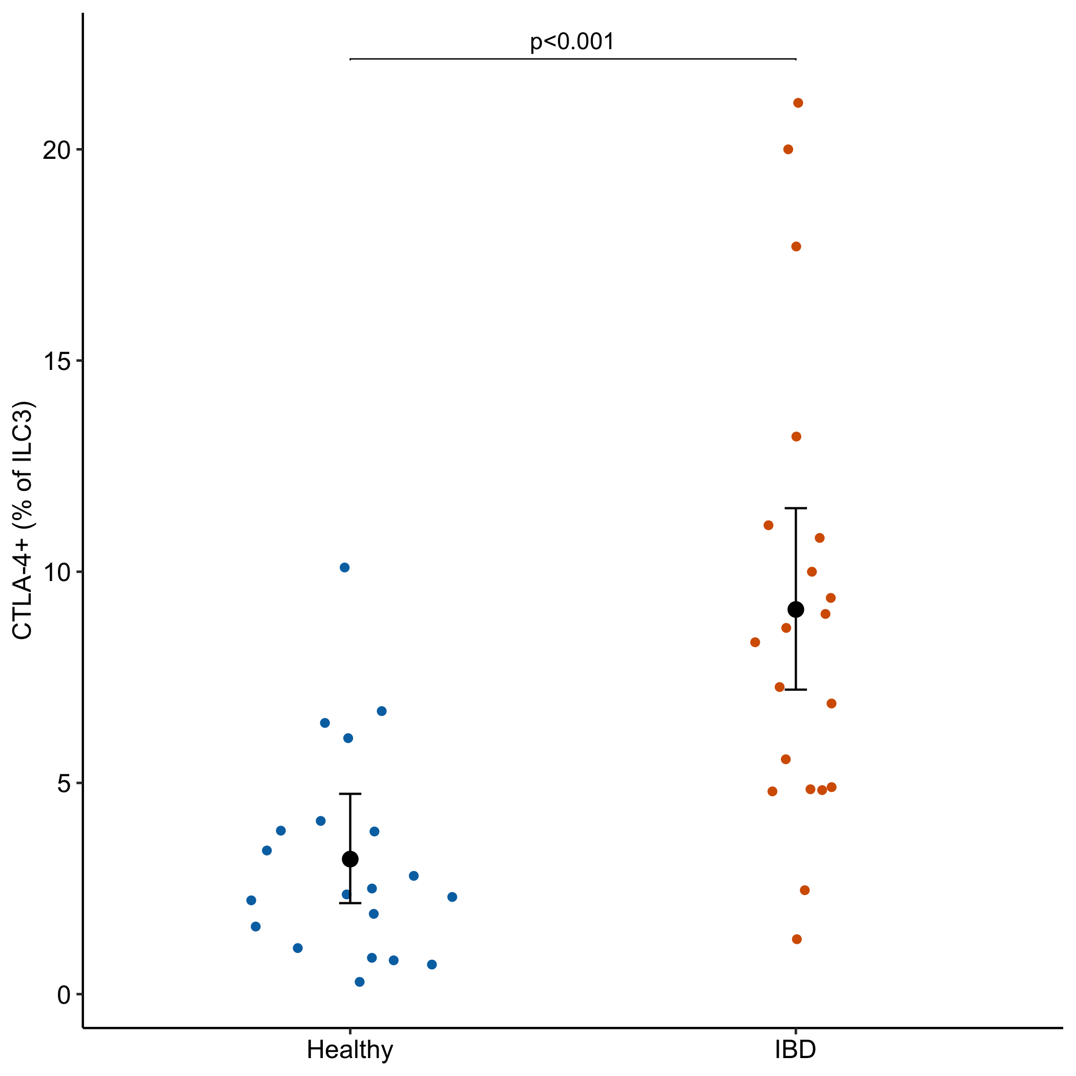
Data From Fig 5c – CTLA-4-expressing ILC3s restrain interleukin-23-mediated inflammation

The data in fig 5c are the percent of a cell subtype relative to all cells of a type, which is a common response variable in bench biology. The researchers analyzed this part-to-whole (a proportion) response with a Mann-Whitney U test. A better practice method is a GLM of the count of the part using the count of the whole as an offset. The effect is the ratio of the treatment proportion relative to the control proportion. This post also shows how to plot the proportion with estimated means and CIs from the GLM with offset model.
percents
proportions
generalized linear model
offset
power
simulation
Author

Jeff Walker

Published

July 5, 2024

Modified

August 18, 2024

Better than Reproducibility of Fig 5c. The CIs and p-values are from a quasipoisson GLM model with offset

Vital info

Data From: Ahmed, A., Joseph, A. M., Zhou, J., Horn, V., Uddin, J., Lyu, M., … & Sonnenberg, G. F. (2024). CTLA-4-expressing ILC3s restrain interleukin-23-mediated inflammation. Nature, 1-8.

Fig: 3k download data

Fig: 5c download data

key words:

Published methods: Mann-Whitney U test

Design: Completely Randomized Design (CRD)

Response: proportion (number of CTLA-4+ ILC3 cells relative to total ILC3 cell count)

Key learning concepts: proportions and offsets

More info: 18.4 Example 2 – Use a GLM with an offset instead of a ratio of some measurement per total (“dna damage” data fig3b)

The Experiment

Intestinal biopsies from patients with IBD versus age- and gender-matched controls

Setup

Import and Wrangle

Code
data_from <- "CTLA-4-expressing ILC3s restrain interleukin-23-mediated inflammation"
file_name <- "41586_2024_7537_MOESM8_ESM.xlsx"
file_path <- here(data_folder, data_from, file_name)

health_levels <- c("Healthy", "IBD")
fig5c <- read_excel(file_path,
                    sheet = "Fig. 5c",
                    range = "F5:G25",
                    col_names = TRUE) |>
  data.table() |>
  melt(variable.name = "health", value.name = "ctla4_pos")
fig5c[, health := factor(health, levels = health_levels)]


file_out_name <- "Fig5c-proportion - CTLA-4-expressing ILC3s restrain interleukin-23-mediated inflammation.xlsx"
fileout_path <- here(data_folder, data_from, file_out_name)
write_xlsx(fig5c, fileout_path)

Reproducibility

Code
wilcox.test(ctla4_pos ~ health, data = fig5c)

    Wilcoxon rank sum exact test

data:  ctla4_pos by health
W = 52, p-value = 2.138e-05
alternative hypothesis: true location shift is not equal to 0

LM

Code
m1 <- lm(ctla4_pos ~ health, data = fig5c)
m1_emm <- emmeans(m1, specs = "health")
m1_pairs <- contrast(m1_emm, method = "revpairwise") |>
  summary(infer = TRUE)
m1_pairs |>
  kable() |>
  kable_styling(full_width = FALSE)
contrast estimate SE df lower.CL upper.CL t.ratio p.value
IBD - Healthy 5.9105 1.33596 38 3.20599 8.61501 4.424158 7.87e-05
Code
ggcheck_the_model(m1)

GLM for percent (proportion of whole) data

Code
fig5c[, ctla4_prop := ctla4_pos/100]
m2 <- glm(ctla4_prop ~ health,
          family = quasibinomial,
          data = fig5c)
m2_emm <- emmeans(m2, specs = "health")
m2_pairs <- contrast(m2_emm, method = "revpairwise") |>
  summary(infer = TRUE)
m2_pairs |>
  kable() |>
  kable_styling(full_width = FALSE)
contrast estimate SE df asymp.LCL asymp.UCL z.ratio p.value
IBD - Healthy 1.110088 0.2486297 Inf 0.622783 1.597393 4.464826 8e-06

Should I use Mann-Whitney, a Linear Model, or a Quasibinomial GLM for proportion data?

Answer: None of the Above

Proportions have strange, non-normal distributions. Samples tend to be right skewed if the mean is closer to zero but left skewed if the mean is closer to 1. And, samples with means closer to 0.5 tend to have more variance than samples closer to 0 or 1. This is probably why the authors used a non-parametric test (Mann-Whitney U). A Mann-Whitney test has higher power than a linear model / t-test but other than the p-value, there are no statistics to plot with the data. There is no effect in a a Mann-Whitney – it is not a test of the differences in the means (or medians!). And, we can’t compute a confidence interval for the group means.

A proportion is a ratio of a part to the whole. A modern statistical method for analyzing proportion data is to use a log-link generalized linear model with the part as the response and the whole as an offset variable. An offset variable is a covariate but the coefficient is forced to be one. By forcing the coefficient to be one, the effect is the ratio of the means of the two proportions (or the difference of the means of the proportions in log space).

GLM for percent (proportion of whole) data when both part and whole are known

The effect (2.85) is the ratio of the mean proportion of the IBD group to the mean proportion of the Health group.

Code
# pretending to have the full count data. Don't do this if you don't have it!
fake_ilc3 <- 432987
fig5c[, ctla4_count := ctla4_pos * 432987]
fig5c[, ilc3_count := 432987]

m3 <- glm(ctla4_count ~ health + offset(log(ilc3_count)),
          family = quasipoisson(link = "log"),
          data = fig5c)
m3_emm <- emmeans(m3, specs = "health", type = "response")
m3_pairs <- contrast(m3_emm, method = "revpairwise") |>
  summary(infer = TRUE)
m3_pairs |>
  kable() |>
  kable_styling(full_width = FALSE)
contrast ratio SE df asymp.LCL asymp.UCL null z.ratio p.value
IBD / Healthy 2.849343 0.6666548 Inf 1.80132 4.507114 1 4.47535 7.6e-06
Code
mean(fig5c[health == "IBD", ctla4_pos])/mean(fig5c[health == "Healthy", ctla4_pos])
[1] 2.849343

A simulation comparing Mann-Whitney, a linear model/t-test, a quasibinomial GLM for proportions, and a quasipoisson GLM with offset

Code
get_clean_proportion_data <- function(n_sample, # sample size
                                      n_cols, # number of samples
                                      mu_num, # numerator
                                      mu_denom, # denominator
                                      theta, # size
                                      rho_matrix, # correlation is in ij
                                      seed_starter){
  fake_y <- rcorrvar(n = n_sample * n_cols,
                     mu = c(mu_num, mu_denom),
                     k_nb = 2,
                     size = c(theta, theta),
                     rho = rho_matrix,
                     seed = seed_starter)$Neg_Bin_variables
  
  n_cols_extra <- n_cols*2
  num_mat <- matrix(fake_y[,"V1"], nrow = n_sample, ncol = n_cols_extra)
  denom_mat <- matrix(fake_y[,"V2"], nrow = n_sample, ncol = n_cols_extra)
  prop_mat <- num_mat/denom_mat
  #cor(ctla4_mat[, 2], ilc3_mat[, 2])

  # check for zero counts
  exc <- NULL
  for(j in 1:n_cols_extra){
    exc_this <- FALSE
    if(any(num_mat[, j] == 0) == TRUE){exc_this <- TRUE}
    if(any(denom_mat[, j] == 0) == TRUE){exc_this <- TRUE}
    if(exc_this == TRUE){
      exc <- c(exc, j)
    }
  }
  if(!is.null(exc)){
    num_mat <- num_mat[, -(exc)]
    denom_mat <- denom_mat[, -(exc)]
    prop_mat <- prop_mat[, -(exc)]
  }
  n_cols_extra <- ncol(num_mat)
  
  # check for prop > 1
  exc <- NULL
  for(j in 1:n_cols_extra){
    exc_this <- FALSE
    if(any(prop_mat[, j] > 1) == TRUE){exc_this <- TRUE}
    if(exc_this == TRUE){
      exc <- c(exc, j)
    }
  }
  if(!is.null(exc)){
    num_mat <- num_mat[, -(exc)]
    denom_mat <- denom_mat[, -(exc)]
    prop_mat <- prop_mat[, -(exc)]
  }
  
  num_mat <- num_mat[, 1:n_cols]
  denom_mat <- denom_mat[, 1:n_cols]
  prop_mat <- prop_mat[, 1:n_cols]
  return(list(
    numerator = num_mat,
    denominator = denom_mat,
    proportion = prop_mat
  ))
}
Code
# get parameters
do_it <- FALSE
if(do_it){
  seed_sim <- 2
  data_params <- fig5c[, .(mean = mean(ctla4_prop),
                           sd = sd(ctla4_prop),
                           N = .N), by = "health"]
  
  # first get theta that approximates that of the data
  do_theta <- FALSE
  if(do_theta){
    n_iter <- 2000
    mu_prop <- data_params$mean
    mu_ctla4 <- mu_prop * 10^5
    mu_ilc3 <- c(10^5, 10^5)
    n_vec <- data_params$N
    rho_ij <- 0.9
    rho_sim <- diag(2)
    rho_sim[1, 2] <- rho_sim[2, 1] <- rho_ij
    theta_vec <- c(0.75, 1, 2)
    sd_table <- data.table(
      set = "fig5c",
      sd_healthy = data_params[1, 3],
      sd_ibd = data_params[2, 3]
    )
    colnames(sd_table) <- c("Set", "SD (Healthy)", "SD (IBD)")
    for(theta_i in theta_vec){
      fake_healthy <- get_clean_proportion_data(
        n_sample = n_vec[1], # sample size
        n_cols = n_iter, # number of samples
        mu_num = mu_ctla4[1], # numerator
        mu_denom = mu_ilc3[1], # denominator
        theta = theta_i, # size
        rho_matrix = rho_sim, # correlation is in ij
        seed_starter = 1)
      fake_ibd <- get_clean_proportion_data(
        n_sample = n_vec[2], # sample size
        n_cols = n_iter, # number of samples
        mu_num = mu_ctla4[2], # numerator
        mu_denom = mu_ilc3[2], # denominator
        theta = theta_i, # size
        rho_matrix = rho_sim, # correlation is in ij
        seed_starter = 2)
      sd_table <- rbind(sd_table,
                        data.table(
                          "Set" = paste("Theta =", theta_i),
                          "SD (Healthy)" = sd(fake_healthy[["proportion"]]),
                          "SD (IBD)" = sd(fake_ibd[["proportion"]])
                        ))
    }    
  }

# results of above show theta = 1 gives a pretty close approximation
# of the SD of the proportions
#             Set SD (Healthy)   SD (IBD)
#          <char>        <num>      <num>
# 1:        fig5c   0.02491151 0.05430466
# 2: Theta = 0.75   0.03697002 0.08533117
# 3:    Theta = 1   0.02506654 0.06500954
# 4:    Theta = 2   0.01250806 0.03550890

  # now do simulation
  # I had abort with n_iter >= 3000 so I'm doing two sets of 2500
  n_iter <- 2500
  iter_sets <- 4
  total_iter <- n_iter * iter_sets
  mu_prop <- data_params$mean
  n_vec <- data_params$N
  rho_ij <- 0.9
  rho_sim <- diag(2)
  rho_sim[1, 2] <- rho_sim[2, 1] <- rho_ij
  theta_i <- 1 # this gives sd of proportions that are close to data. see above simulation

  fd <- data.table(
    health = rep(c("Healthy", "IBD"), data_params$N),
    ilc3 = as.numeric(NA),
    ctla4 = as.numeric(NA)
  )
  
  power_matrix <- matrix(nrow = total_iter, ncol = 5)
  colnames(power_matrix) <- c("mwu","lm", "qb", "nb", "qp")
  type1_matrix <- matrix(nrow = total_iter, ncol = 5)
  colnames(type1_matrix) <- c("mwu","lm", "qb", "nb", "qp")

  seed_starter_sim <- 0
  for(iter_set in 1:iter_sets){
    seed_starter_sim <- seed_starter_sim + 1
    # power
    # make effect size smaller so power < 1
    mu_prop[2] <- mu_prop[1] * 1.5
    mu_ctla4 <- mu_prop * 10^5
    mu_ilc3 <- c(10^5, 10^5)
    fake_healthy <- get_clean_proportion_data(
      n_sample = n_vec[1], # sample size
      n_cols = n_iter, # number of samples
      mu_num = mu_ctla4[1], # numerator
      mu_denom = mu_ilc3[1], # denominator
      theta = theta_i, # size
      rho_matrix = rho_sim, # correlation is in ij
      seed_starter = seed_starter_sim)
    
    seed_starter_sim <- seed_starter_sim + 1
    fake_ibd <- get_clean_proportion_data(
      n_sample = n_vec[2], # sample size
      n_cols = n_iter, # number of samples
      mu_num = mu_ctla4[2], # numerator
      mu_denom = mu_ilc3[2], # denominator
      theta = theta_i, # size
      rho_matrix = rho_sim, # correlation is in ij
      seed_starter = seed_starter_sim)
    ctla4_mat <- rbind(fake_healthy[["numerator"]],
                       fake_ibd[["numerator"]])
    ilc3_mat <- rbind(fake_healthy[["denominator"]],
                      fake_ibd[["denominator"]])
    ctla4_prop_mat <- rbind(fake_healthy[["proportion"]],
                            fake_ibd[["proportion"]])
    
    for(iter in 1:n_iter){
      sim_i <- n_iter*(iter_set - 1) + iter
      # fake data
      fd[, ctla4 := ctla4_mat[, iter]]
      fd[, ilc3 := ilc3_mat[, iter]]
      fd[, ctla4_prop := ctla4_prop_mat[, iter]]
      
      # Mann Whitney
      power_matrix[sim_i, "mwu"] <- wilcox.test(ctla4_prop ~ health, data = fd)$p.value
      
      # lm
      m_lm <- lm(ctla4_prop ~ health, data = fd)
      power_matrix[sim_i, "lm"] <- coef(summary(m_lm))["healthIBD", "Pr(>|t|)"]
      
      # glm bin
      m_qb <- glm(ctla4_prop ~ health,
                  family = quasibinomial,
                  data = fd)
      power_matrix[sim_i, "qb"] <- coef(summary(m_qb))["healthIBD", "Pr(>|t|)"]
      
      # glm nb
      m_nb <- glm.nb(ctla4 ~ health + offset(log(ilc3)),
                     data = fd)
      power_matrix[sim_i, "nb"] <- coef(summary(m_nb))["healthIBD", "Pr(>|z|)"]
      
      # glm qp
      m_qp <- glm(ctla4 ~ health + offset(log(ilc3)),
                  family = quasipoisson(link = "log"),
                  data = fd)
      power_matrix[sim_i, "qp"] <- coef(summary(m_qp))["healthIBD", "Pr(>|t|)"]
      
      #       do_plot <- FALSE
      #       if(do_plot){
      #         m_qb_emm <- emmeans(m_qb, specs = "health", type = "response")
      #         m_qb_pairs <- contrast(m_qb_emm, method = "revpairwise") |>
      #           summary(infer = TRUE)
      # #        plot_response(m_qb, m_qb_emm, m_qb_pairs)
      #         ggplot(data = fd,
      #                aes(x = health,
      #                    y = ctla4_prop,
      #                    color = health)) +
      #           geom_point()
      #       }
      
    }
    
    
    # type I
    mu_prop[2] <- mu_prop[1]
    mu_ctla4 <- mu_prop * 10^5
    mu_ilc3 <- c(10^5, 10^5)
    
    seed_starter_sim <- seed_starter_sim + 1
    fake_healthy <- get_clean_proportion_data(
      n_sample = n_vec[1], # sample size
      n_cols = n_iter, # number of samples
      mu_num = mu_ctla4[1], # numerator
      mu_denom = mu_ilc3[1], # denominator
      theta = theta_i, # size
      rho_matrix = rho_sim, # correlation is in ij
      seed_starter = seed_starter_sim)
    seed_starter_sim <- seed_starter_sim + 1
    fake_ibd <- get_clean_proportion_data(
      n_sample = n_vec[2], # sample size
      n_cols = n_iter, # number of samples
      mu_num = mu_ctla4[2], # numerator
      mu_denom = mu_ilc3[2], # denominator
      theta = theta_i, # size
      rho_matrix = rho_sim, # correlation is in ij
      seed_starter = seed_starter_sim)
    ctla4_mat <- rbind(fake_healthy[["numerator"]],
                       fake_ibd[["numerator"]])
    ilc3_mat <- rbind(fake_healthy[["denominator"]],
                      fake_ibd[["denominator"]])
    ctla4_prop_mat <- rbind(fake_healthy[["proportion"]],
                            fake_ibd[["proportion"]])
    
    for(iter in 1:n_iter){
      sim_i <- n_iter*(iter_set - 1) + iter
      # fake data
      fd[, ctla4 := ctla4_mat[, iter]]
      fd[, ilc3 := ilc3_mat[, iter]]
      fd[, ctla4_prop := ctla4_prop_mat[, iter]]
      
      # Mann Whitney
      type1_matrix[sim_i, "mwu"] <- wilcox.test(ctla4_prop ~ health, data = fd)$p.value
      
      # lm
      m_lm <- lm(ctla4_prop ~ health, data = fd)
      type1_matrix[sim_i, "lm"] <- coef(summary(m_lm))["healthIBD", "Pr(>|t|)"]
      
      # glm bin
      m_qb <- glm(ctla4_prop ~ health,
                  family = quasibinomial,
                  data = fd)
      type1_matrix[sim_i, "qb"] <- coef(summary(m_qb))["healthIBD", "Pr(>|t|)"]
      
      # glm nb
      m_nb <- glm.nb(ctla4 ~ health + offset(log(ilc3)),
                     data = fd)
      type1_matrix[sim_i, "nb"] <- coef(summary(m_nb))["healthIBD", "Pr(>|z|)"]
      
      # glm qp
      m_qp <- glm(ctla4 ~ health + offset(log(ilc3)),
                  family = quasipoisson(link = "log"),
                  data = fd)
      type1_matrix[sim_i, "qp"] <- coef(summary(m_qp))["healthIBD", "Pr(>|t|)"]
      
    }    
  }

  saveRDS(power_matrix, "power_matrix.Rds")
  saveRDS(type1_matrix, "type1_matrix.Rds")
}else{
  power_matrix <- readRDS("power_matrix.Rds")
  type1_matrix <- readRDS("type1_matrix.Rds")
}

pless <- function(x, alpha = 0.05){
  stat <- sum(x <= alpha)/length(x)
  return(stat)
}
Code
res <- data.table(
  Test = c("Mann-Whitney", "Linear Model/T-test", "Quasibinomial", "Negative Binomial", "Quasipoisson"),
  Power = apply(power_matrix, 2, pless, alpha = 0.05),
  "Type I" = apply(type1_matrix, 2, pless, alpha = 0.05)
)
res |>
  kable(digits = c(1,2,3)) |>
  kable_styling(full_width = FALSE)
Test Power Type I
Mann-Whitney 0.69 0.047
Linear Model/T-test 0.56 0.040
Quasibinomial 0.58 0.046
Negative Binomial 0.70 0.106
Quasipoisson 0.83 0.075

For data that look like those in fig. 5c, the Mann-Whitney has good Type I control and high power relative to the linear model/t-test and compared to the quasibinomial GLM model. But the quasipoisson GLM offset model for the original counts has 20% higher power than the Mann-Whitney, but slightly elevated Type 1. And the beauty of the quasipoisson GLM is we get model statistics to plot with the data (see the plot below).

The table below shows the Power and Type I error when alpha is set to 0.03. The power for the quasipoisson model with alpha = 0.03 has good Type I control and is 13% higher than the power for the Mann-Whitney with alpha = 0.05.

Code
res <- data.table(
  Test = c("Mann-Whitney", "Linear Model/T-test", "Quasibinomial", "Negative Binomial", "Quasipoisson"),
  Power = apply(power_matrix, 2, pless, alpha = 0.03),
  "Type I" = apply(type1_matrix, 2, pless, alpha = 0.03)
)
res |>
  kable(digits = c(1,2,3)) |>
  kable_styling(full_width = FALSE)
Test Power Type I
Mann-Whitney 0.61 0.027
Linear Model/T-test 0.47 0.022
Quasibinomial 0.49 0.027
Negative Binomial 0.64 0.072
Quasipoisson 0.78 0.047

If using the quasipoisson GLM we could make the test a bit more conservative by using smaller alpha, but again, I don’t think bench biologists really use alpha in any formal sense.

Plot the model

A good question is, how do we Plot the Model? A proportion response makes sense for communication but the emmeans table has whole-count adjusted counts as the mean response. But these adjusted counts are proportions, just unscaled by the denominator. So we can rescale the mean and CIs as proportions (or percents) by dividing by the mean counts of the whole (ilc3 count).

Code
m3_emm_dt <- m3_emm |>
  summary() |>
  data.table()
m3_pairs_dt <- data.table(m3_pairs)

# rescale mean and CIs to percent
means_table <- fig5c[, .(ctla4 = mean(ctla4_count),
                         ilc3 = mean(ilc3_count),
                         ctla4_per = mean(ctla4_pos)), by = health]
scale_factor <- mean(fig5c$ilc3)
m3_emm_dt[, mean :=rate/scale_factor]
m3_emm_dt[, lo :=asymp.LCL/scale_factor]
m3_emm_dt[, hi :=asymp.UCL/scale_factor]

gg <- ggplot(data = fig5c,
             aes(x = health,
                 y = ctla4_pos,
                 color = health)) +
  geom_sina(maxwidth = 0.5,
            show.legend = FALSE) +
  geom_errorbar(data = m3_emm_dt,
                aes(x = health,
                    y = mean,
                    ymin = lo,
                    ymax = hi),
                width = 0.05,
                color = "black") +
  geom_point(data = m3_emm_dt,
             aes(x = health,
                 y = mean),
             size = 3,
             color = "black") +
  ylab("CTLA-4+ (% of ILC3)") +
  scale_color_manual(values = pal_okabe_ito_2) +
  theme_pubr() +
  theme(axis.title.x = element_blank()) +
  NULL

  # add p-values
m3_pairs_dt[, group1 := "Healthy"]
m3_pairs_dt[, group2 := "IBD"]
m3_pairs_dt[, p := p.value |>
              p_round(digits = 2) |>
              p_format(digits = 2, accuracy = 1e-03, add.p = TRUE)]
maxy <- fig5c[, max(ctla4_pos)]
miny <- fig5c[, min(ctla4_pos)]
m3_pairs_dt[, y.position := maxy + 0.05*(maxy - miny)]

gg <- gg +
  stat_pvalue_manual(
    data = m3_pairs_dt,
    label = "p",
    tip.length = 0.001)

gg

Code
save_it <- FALSE
if(save_it){
out_fig <- "fig5c_ggplot.png"
out_path <- here("figs", data_from, out_fig)
ggsave(out_path)
}